Are you tired of scrolling through endless rows and columns in Excel? Look no further!
In this article, we’ll show you how to freeze columns and rows using the powerful Freeze Panes feature. With our step-by-step guide, you’ll be able to easily navigate through your spreadsheets without losing sight of important data.
Whether you’re a beginner or an advanced user, we’ve got you covered with troubleshooting tips and advanced techniques.
Let’s get started and make your Excel experience a breeze!
Understanding the Freeze Panes Feature
Understanding the freeze panes feature allows you to keep certain columns and rows visible while scrolling in Excel. This feature is extremely useful when working with large spreadsheets that require constant scrolling. By freezing panes, you can keep important information, such as headers or labels, static while navigating through the rest of the data.
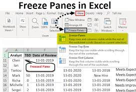
To freeze panes, simply select the column or row where you want the freeze to begin, and then go to the View tab and click on the Freeze Panes option. This will ensure that the selected column or row, along with all the ones above and to the left of it, remain visible at all times.
With the freeze panes feature, you can effortlessly navigate through your spreadsheet without losing sight of critical data.
Step-by-Step Guide to Freezing Columns in Excel
To keep specific information visible while scrolling, you’ll want to make sure you lock certain parts of your spreadsheet in place. Freezing columns in Excel is a handy feature that allows you to keep certain columns visible while you navigate through your data.
Here’s a step-by-step guide to help you freeze columns in Excel.
- Select the column that you want to freeze.
- Go to the ‘View’ tab and click on the ‘Freeze Panes’ button.
- From the dropdown menu, choose ‘Freeze Panes’.
- You will notice a gray line appear on the left side of your selected column, indicating that it is now frozen.
- Now, as you scroll horizontally, the frozen column will remain visible.
- This makes it easier to compare data and analyze information without losing track of important columns.
How to Freeze Rows in Excel: A Comprehensive Tutorial
When working with large data sets in Excel, you’ll find it helpful to keep specific information at the top of your view while scrolling. Freezing rows in Excel allows you to do just that.
To freeze rows, first, select the row below the one you want to freeze. For example, if you want to freeze the first row, select the second row.
Next, go to the View tab and click on Freeze Panes. From the drop-down menu, select Freeze Panes again.
Now, when you scroll down, the frozen row will remain at the top of your view, making it easy to reference important information.
Freezing rows is especially useful when working with large datasets that require constant referencing of column headers or other specific information.
Advanced Techniques for Freezing Columns and Rows
By adjusting the frozen area, you can customize your view to focus on the most relevant information.
In Excel, freezing columns and rows is a powerful technique that allows you to keep important data visible at all times, even when scrolling through a large spreadsheet.
To freeze columns, simply select the column to the right of the ones you want to freeze, and then click on the ‘View’ tab. From there, click on the ‘Freeze Panes’ button and select ‘Freeze Panes’ from the drop-down menu. This will freeze all columns to the left of the selected column.
Similarly, to freeze rows, select the row below the ones you want to freeze and follow the same steps.
Troubleshooting and Tips for Freezing Panes in Excel
For a smoother experience, make sure you select the correct column or row when freezing panes in Excel.
Sometimes, you might find that the frozen panes are not working as expected. In such cases, there are a few troubleshooting steps you can try.
First, check if you have selected the correct cell before freezing the panes. If you’ve selected a cell outside the desired column or row, the freezing won’t work properly.
Additionally, ensure that you haven’t accidentally selected multiple columns or rows when freezing. This can cause confusion and prevent the freezing from functioning correctly.
Lastly, make sure that the worksheet isn’t protected, as freezing panes might not be allowed in protected sheets.
Conclusion
In conclusion, freezing columns and rows in Excel can greatly enhance your data analysis experience. By using the Freeze Panes feature, you can keep important information visible while scrolling through large spreadsheets.
Whether you need to freeze columns or rows, this comprehensive tutorial has provided you with step-by-step instructions. Additionally, we have covered advanced techniques and troubleshooting tips to ensure smooth usage of this feature.
So go ahead and make use of this powerful tool to make your Excel worksheets more organized and user-friendly.