Are you tired of constantly scrolling through your Google Sheets to find important information?
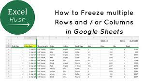
In this article, we will show you how to freeze a row in Google Sheets, making your data easily accessible at all times.
By following our step-by-step guide, you will learn how to take advantage of this handy feature and save yourself valuable time.
Say goodbye to endless scrolling and hello to a more efficient way of working with your spreadsheets!
Why Freeze Rows in Google Sheets
Why don’t you freeze rows in Google Sheets to keep important information always visible?
Freezing rows in Google Sheets allows you to lock certain rows at the top of your spreadsheet, so they stay in place while you scroll through the rest of your data.
This is especially useful when you have a large dataset and need to reference specific information in a particular row. By freezing rows, you can ensure that important headers, titles, or formulas are always visible, making it easier to navigate and analyze your data.
Whether you’re working on a budget spreadsheet, tracking sales data, or organizing a project plan, freezing rows in Google Sheets can save you time and help you stay focused on the most relevant information.
Understanding the Benefits of Freezing Rows in Google Sheets
Understanding the advantages of freezing rows in Google Sheets can greatly enhance your productivity.
When you freeze a row, it stays fixed at the top of your sheet, even as you scroll down. This feature is especially useful when working with large datasets or long lists, as it allows you to keep important information in view at all times.
By freezing the header row, for example, you can easily refer to column labels while navigating through your data. Freezing rows also comes in handy when you need to compare data in different sections of your sheet. Instead of constantly scrolling back and forth, you can keep relevant rows visible and make quick comparisons.
With freezing rows, you can work more efficiently and save valuable time.
Step-by-Step Guide to Freezing Rows in Google Sheets
To start, it’s essential to know the step-by-step process of how to freeze specific rows in your Google Sheets.
First, open your Google Sheets document and locate the row that you want to freeze.
Next, click on the row number to select the entire row.
Then, navigate to the ‘View’ menu and click on ‘Freeze’ followed by ‘2 rows’ to freeze the selected row and the row above it.
If you want to freeze more than two rows, simply select the desired number of rows and choose the ‘Freeze’ option accordingly.
Once you’ve frozen the desired rows, you can scroll through your spreadsheet while keeping those rows visible at all times.
That’s it! Now you know how to easily freeze specific rows in your Google Sheets.
Troubleshooting Common Issues When Freezing Rows in Google Sheets
If you’re having trouble with freezing rows in Google Sheets, one common issue could be not selecting the correct number of rows to freeze.
When you freeze rows in Google Sheets, it allows you to keep certain rows visible while scrolling through large datasets.
To freeze rows, you need to select the row below the rows you want to freeze. For example, if you want to freeze the first three rows, you should select the fourth row.
If you mistakenly select the wrong row or a larger number of rows, it can cause freezing issues. So, make sure you carefully select the correct number of rows to freeze to avoid any problems.
Advanced Techniques for Freezing Rows in Google Sheets
One helpful technique for freezing specific sections in Google Sheets is by using the ‘View’ menu.
To freeze a row in Google Sheets, first, select the row that you want to freeze by clicking on the row number.
Then, go to the ‘View’ menu at the top of the screen and click on ‘Freeze’. A drop-down menu will appear, and you can choose to freeze either the selected row or the first row.
Conclusion
In conclusion, freezing rows in Google Sheets is a simple yet powerful feature that can greatly enhance your spreadsheet experience. By following the step-by-step guide provided, you can easily freeze rows and keep important information visible as you scroll through your data.
And if you encounter any issues, the troubleshooting tips will help you resolve them quickly. With the advanced techniques, you can further customize your frozen rows and optimize your workflow.
So go ahead and take advantage of this handy feature in Google Sheets to make your work more efficient.